Random Variables and Distributions
We will be briefly look at some concepts which are useful when working with sample spaces, especially large sample spaces.
Random Variables
Let $S$ be a sample space. We want to associate a value to each element of the sample space. We can do that using a function $$X:S\rightarrow \mathbb{R}$$ which is (unfortunately) called a random variable. Here are some examples of sample spaces $S$ with random variables $X$:
- $S$ is $1$ coin toss, and $X=1$ for heads and $X=0$ for tails.
- $S$ is $10$ coin tosses, and $X$ counts the number of heads.
- $S$ is the people in this class, and $X$ is a student's height.
- $S$ is rolling one dice, and $X$ is the value shown.
- $S$ is rolling three dice, and $X$ is the sum of the values shown.
- $S$ are all movements in a maze starting at a fixed location, and $X$ is the number of moves until the exit is found.
- $S$ are all (one-player) gameplays of the game "snakes and ladders", and $X$ is the number of rolls until the game is finished.
- $S$ are all (one-player) gameplays of the game "Yahtzee", and $X$ is the final score.
Like other functions, random variables can be combined in various ways to form new random variables. For instance you can add and multiply random variables, and you can multiply a random variable with a scalar.
From a random variable $X$ and $x\in \mathbb{R}$ you can create the event $\{s\in S|X(s)=x\}$ of all outcomes where $X$ take the value $x$. These events have associated probabilities, which are denoted by $$p_X(x) \mbox{ or }P(X=x).$$ The collection of all these probabilities is called the distribution of $X$. The function $$p_X:\mathbb{R}\rightarrow \mathbb{R}$$ is called the probability function of $X$.
From each event $A$ in a sample space $S$ we can construct a random variable $X$ with $X(s)=1$ if $s\in A$ and $X(s)=0$ if $s\not \in A$. For this random variable we the distribution $$p_X(0)=P(\overline{A} \mbox{ and } p_X(1)=P(A).$$
Finally, two random variables $X$ and $Y$ are independent, if $$P(X=x\wedge Y=y)=p_X(x)\cdot p_Y(y).$$ Similar to independent events, the interpretation of independence is that information about the value of $X$ tells us nothing about the value of $Y$, and vice versa.
An example
Lets look at an example. Let $S$ be the outcome of rolling three dice and let $X$ be the sum of the values. Describe the distribution of $X$.
In this example, $X$ can take any value $3, 4, \cdots, 18$. We have the following table of probabilities computed with Python. Note that I write $216$ times the probability in order to avoid fractions.
$$\begin{matrix} x && 216\cdot p(x) \\ \\ 3 && 1 \\ 4 && 3 \\ 5 && 6 \\ 6 && 10 \\ 7 && 15 \\ 8 && 21 \\ 9 && 25 \\ 10 && 27 \end{matrix} \begin{matrix} x && 216\cdot p(x) \\ \\ 11 && 27\\ 12 && 25\\ 13 && 21\\ 14 && 15\\ 15 && 10\\ 16 && 6\\ 17 && 3\\ 18 && 1 \end{matrix}$$
We can also draw a histogram, for instance by typing
import matplotlib.pyplot as plt
plt.hist([i+j+k for i in range(1,7) \
for j in range(1,7) for k in range(1,7)],16)
in Python.
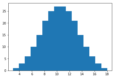
Note that the plot reveals a clearly defined middle, with other values spreading out and decreasing away from the middle. This is a pattern you will see in many distributions.
We will now define precise quantities which compute the middle and the spread of any distribution - without relying on tables or plots.
Expectation
The expectation (or mean) of a random variable is $$E(X) = \sum x p_X(x) = \sum x P(X = x)$$
The law of large numbers says that if you draw $n$ random samples from $S$, then the average value $$m=\frac{1}{n}(X_1+X_2+\cdots X_n)$$ approaches $E(X)$ when $n\rightarrow \infty$. Here $X_i$ is the value we obtain on the $i$'th draw. So the expectation should be thought of as the average value of $X$. It is one way of giving a precise definition of the middle of the histogram plot of the distribution.
We have $$E(aX+bY)=aE(X)+bE(Y)$$ for scalars $a$ and $b$ and random variables $X$ and $Y$. We also have $$E(g(X))=\sum g(x) p_X(x)$$ for (in our case) all functions $g:\mathbb{R}\rightarrow \mathbb{R}$. This formula is called the law of the unconscious statistician or LOTUS.
If you are working with data, you may not have complete information about the distribution. If so, you can estimate (i.e. approximate) the mean by selecting a large random subset of the sample space, and compute the average of the values $$m=\frac{1}{n}\sum_i X_i$$ of your data. If the data set was chosen large enough, then $m$ should be a good approximation of the mean $E(X)$.
Examples
What is the expected value of the value shown on the dice when we roll one dice.
Let $X$ be the random variable showing the value on a rolled dice. We have $$E(X)=\sum_{i=1}^6 \frac{1}{6} \cdot i = 3.5$$ The example illustrates the important point that $E(X)$ is not necessarily one of the values taken by $X$.
We play a game where we roll one dice. If we roll even, we pay the opponent $1$ coin. If we roll odd, the opponent pays us $2$ coins. What is the expected amount of coins we will get with one roll of the dice.
Let $X$ be the random variable with value $2$ if the dice rolls odd and $-1$ if the dice rolls even. So $X$ measures our earnings on one roll of the dice. We have $$E(X) = \frac{1}{2}\cdot 2 + \frac{1}{2}\cdot (-1) = 0.5.$$ So on one roll of the dice we should expect to be paid (on average) $0.5$ coins.
You play a game with one dice. If you roll an even number you pay $1$ coin to the opponent. If you roll an odd value you get $2$ coins from the opponent. What is the expected amount of coins paid to you after $n$ rolls of the dice
Let $X_i$ be $2$ if you roll odd on the $i$'th roll, and $X_i=-1$ if you roll even. With $n$ rolls you should expect to win $E(X_1+\cdots+X_n) = 0.5n$ coins. In a game of chance, where $X$ measures earnings, $E(X)$ tells us something about earnings over time. The actual payout could vary widely in the short term however.
We roll $3$ dice and let $X$ be the random variable computing the sum of the values. What is the expected value of $X$
As above let $X_i$ be the value shown on the $i$'th dice. Then we need to compute $E(Y)$ for $Y=X_1+X_2+X_3$, which is $$E(Y)=3\cdot E(X)=3\cdot 3.5 = 10.5.$$ We could also (with a lot more work) calculate $E(Y)$ directly, $$E(Y)=\frac{1}{216}(3\cdot 1 + 4\cdot 3 + \cdots + 17\cdot 3 + 18\cdot 1)$$ to obtain the same result.
We look at another example. The sample space is outcomes of rolling $6$ dice. Let $X$ be the random variable which computes the sum of the dice. Let us compute the expectation of $X$ using three different approaches.
First the expected value for a roll of one dice is $3.5$. The expected sum of six roll of the dice will then be $$E(X_1+\cdots+X_6)=6\cdot 3.5 = 21.$$ We should not expect the calculation to be so easy for all problems, so lets explore a few more possible approaches we could have taken.
We create a list of the whole sample space, and use the definition of $E(X)$. This would require a computer, as the sample space has $6^6=46656$ elements. In Python we could do:
import itertools as it
r = range(1,7)
sample = list(it.product(r,r,r,r,r,r))
diceSums = list(map(lambda x : sum(x), sample))
print(sum(diceSums) / len(sample))
We again get the number $21$
If the problem was such that listing all the elements was impossible, we could also run a simulation (more about simulations in the next section).
import random as rnd
numSample = 10000
rnd.seed()
totalsum = 0
for i in range(numSample):
roll = (rnd.randint(1,6) for d in range(6))
totalsum += sum(roll)
print(totalsum / numSample)
When I ran the code I got $20.9369$, which is a reasonable approximation of the correct value $21$.
Variance
So we have found the average value (or expected value) of $X$, as a way of defining the middle of a general distribution. We now want to say something about how the values of $X$ are spread out around it's average. To do that we introduce the variance of $X$: $$Var(X) = E((X-\mu)^2) = E(X^2) - E(X)^2$$ where $E(X^2)=\sum x^2f(x)$ by LOTUS. The variance measures the spread of $X$., i.e. the tendency for values of $X$ to be far away from the average $E(X)$. If the variance is very small, then typical values of $X$ will be very close to $E(X)$. If the variance is large, then typical values of $X$ will be spread out on both sides of $E(X)$ on the number line.
One problem with variance is that it is not measured in the same units as the variables $X$. For instance if $X$ is measured in meters, then the variance is measured in meters squared. To remedy that we can instead use the standard deviation $$\sigma_X = \sqrt{Var(X)}$$ which does have the same unit of measurement as $X$.
If $X_i$ are independent random variables, then $$Var(X_1+X_2+\cdots+X_n)= Var(X_1)+Var(X_2)+\cdots+Var(X_n).$$ This is different from the corresponding formula for the mean, where independence is not required. Also, $$a^2Var(X)=Var(aX)$$ for any scalar $a$.
Examples
We roll one six-sided fair dice. What is the variance and standard deviation of the value shown on the dice?
Let $X$ be the random variable showing the value on a rolled dice. Having already computed the expected value of $X$, we get $$E(X)^2=\frac{49}{4}$$ $$E(X^2)=\frac{1}{6}(1+4+9+16+25+36)=\frac{91}{6}$$ and so the variance is $$Var(X)=E(X^2)-E(X)^2\approx 2.92$$ and the standard deviation is $\sigma_X\approx 1.71$.
Let us go back to our game of dice, where we receive $2$ coins on an odd roll and pay $1$ coin on an even roll. What is the variance and standard deviation of coins paid to you in one roll of the dice.
We have $E(X)^2=\frac{1}{4}$ and $E(X^2)=\frac{1}{2}\cdot 4 + \frac{1}{2}\cdot 1 = \frac{5}{2}$ and so $$Var(X)=\frac{5}{2}-\frac{1}{4}=\frac{9}{4}$$ and $$\sigma_X = 1.5.$$
What is the variance after $100$ rolls.
Let $X_i$ be $2$ if you roll odd on the $i$'th roll, and $X_i=-1$ if you roll even. With $n$ rolls the variance is $Var(X_1+\cdots+X_n) = Var(X_1)+Var(X_2)+\cdots+Var(X_n)=\frac{9}{4}n$ and the standard deviation is $$\sigma_X = 1.5\sqrt{n}.$$ So for instance after $100$ rolls the expected earnings is $50$ with standard deviation $15$.
Estimating variance
Note that, if we only have partial knowledge of the distribution of $X$, but know the mean $E(X)$, we can estimate the variance by computing the average $$\frac{1}{n}\sum_i(X_i - E(X))^2$$ over the data set $X_i$.
If we have estimated the mean as well, then you should use $$\frac{1}{n-1}\sum_i(X_i - m)^2.$$ The explanation for this last formula is outside the scope of this course.
Lets again consider the example of the variance of the sum of the roll of six dice. We can compute the variance directly as $17.5$. We see that using the formula $Var(\sum_i X_i)=\sum_i Var(X_i)$ for independent rolls $X_i$ of one dice (computed above). Nevertheless, lets look at some other methods for finding the variance which are applicable in situations where computations are not so straightforward.
We can calculate the exact value of the variance by summing over the whole sample space. This will work as long as the sample space is not too large.
r = range(1,7)
sample = list(it.product(r,r,r,r,r,r))
diceSums = list(map(lambda x : sum(x), sample))
expt = sum(diceSums) / len(sample)
var = sum(map(lambda x : (x-expt)**2 ,diceSums))/len(sample)
Given that we know the expectation to be $21$, we can also simulate to find an approximation to the variance in this way
numSample = 1000000
rnd.seed()
totalsum = 0
for i in range(numSample):
roll = [rnd.randint(1,6) for d in range(6)]
totalsum += (sum(roll)-21)**2
variance = totalsum / numSample
The Chebyshev Inequality
We now use the standard deviation to be more precise about the spread of values of $X$. A simple approach is using the Chebyshev Inequality. Assume we know mean $E(X)$ and the standard deviation, then $$P(|X-E(X)|\geq t) \leq \frac{Var(X)}{t^2}$$
Imagine playing a game of chance. You know that your expected earnings is $500$ and that the variance is $250$. It does not matter what the rules of the games are, or how we came to find the expectation and variance. The Chebuyshev inequality now says: $$P(|X-500|\geq t)\leq \frac{250}{t^2}$$
Find a bound on the probability that our earnings will be $500\pm 100$?
Without knowing more about the game (i.e. the distribution of the earning $X$) it would be impossible to calculate the exact probability in this question. We can however use the Chebuyshev inequality to find a bound. The inequality says $$P(|X-500|\geq 100)\leq \frac{250}{100\cdot 100} = 0.025.$$ So whatever the actual probability is, it is certainly less than $2.5$ per cent. The power of this bound is that it is valid no matter how the game is played.
Find $x$ so that it is at least $90$ per cent certain that our earnings will be $500\pm x$.
We want $$P(|X-500|\geq t)\leq \frac{250}{t^2}=1-0.9=0.1$$ and need to find $t$. We solve $$\frac{250}{t^2}=0.1\mbox{ and get }t=50.$$ So we can be $90$ per cent certain that our earnings will be $500\pm 50$. Again the real power of this bound is that is does not matter how the game is played.
The Chebyshev bound is usually quite loose, and we can do better if we know more about the distribution of $X$. However, we will not discuss these matters further in this course. We will look more at this inequality when we discuss simulations.
Covariance
This section will be needed to get a deeper understanding some of the material in module 3. How much of this material we will be needing depends on the type of examples we will be doing, and that is not decided at the moment, so you can skip this section for now.
The covariance of $X$ and $Y$ is defined by $$Cov(X,Y)=E((X-E(X))\cdot (Y-E(Y)))$$ The covariance is a measure of the linear relationship between $X$ and $Y$. We have:
- $Cov(X,Y) > 0$: $Y$ is large/small when $X$ is large/small.
- $Cov(X,Y) < 0$: $Y$ is small/large when $X$ is large/small.
- $Cov(X,Y) = 0$: No linear relation between $X$ and $Y$.
We would like to measure how strong the relationship is between $X$ and $Y$. To do that we can normalise the covariance to take values between $-1$ and $1$ by introducing the correlation of $X$ and $Y$: $$\rho(X,Y) = \frac{Cov(X,Y)}{\sigma_X \sigma_Y}$$ If $|\rho(X,Y)|$ is close to $1$, then there is a strong relationship between $X$ and $Y$. If $|\rho(X,Y)|$ is close to $0$, then there is a weak relationship.
The concept of correlation is sometimes misused. One common mistake is to assume that correlation implies causation.
Correlation does not imply causation: Positive or negative correlation does not mean that changing $X$ causes $Y$ to change or vice versa.
The Bernoulli distribution
There are many distributions that occur often enough to have been given names. Usually there are precomputed values for expectation and variance for these distributions. We will look at one of them.
You have a sample space $S$ where each element has equal probability of being drawn. The sample space is divided into elements of two types; those which have some property $A$, and those which do not have property $A$. We can think of $A$ as an event with some probability $P(A)=p$. We want to express $E(X)$ and $Var(X)$ in terms of this probability.
A random variable $X$ is said to have the Bernoulli distribution if it takes the value $1$ if an element with property $A$ is drawn and value $0$ if an element without the property $A$ is drawn. In applications you will often find that $0/1$ represents true/false, yes/no, success/failure, etc.
The probability function is given by $$p_X(x)=p,$$ the mean is $p$ and the variance is $p(1-p)$. Note that the variance is always smaller than $\frac{1}{4}$, independent of $p$.