Markov Chains

We are now going to use simple weighted networks and matrices to study probabilities. In this context, nodes are called states, and weights on the arrows encode probabilities of moving between states.

We start with a network the following two properties:

Each weight is a probability, i.e. in the interval $(0,1]$
The sum of weights on arrows leaving a state is equal to $1$.

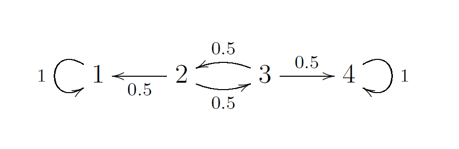
Note that there are no restrictions on the weights going into a state and we do not draw arrows with weight $0$. Here is an example of such a network with $4$ states.

Recall that networks can be represented with matrices. The corresponding properties for matrices are

Entries in the matrix are probabilities, i.e. in the interval $[0,1]$
The sum of values in any column is equal to $1$.

Such a matrix is called a stochastic matrix. Note that there is no restriction on the sum of values in rows. The matrix for the example above is $$P=\begin{pmatrix}1 & 0.5 & 0 &0 \\ 0 & 0 & 0.5 & 0 \\ 0 & 0.5 & 0 & 0 \\ 0 & 0 & 0.5 & 1\end{pmatrix}$$ where we choose the ordering of rows/columns by the labels in the picture. We could have chosen another ordering which would give us another transition matrix for the chain.

Given such a network (or a stochastic matrix) we can perform a random walk according to the following rule: Assume that our current state is $i$ and we want to move to the next state. We choose one of the arrows going out of the state. This choice is made randomly, with probability equal to the weight on the arrow. Once the arrow is chosen, we can follow that arrow to the next state.

Note that the change of state depends only on the state we are located at, and not how we arrived at that state. A random walk with this property is said to have the Markov property or is called memoryless. Such a network together with these rules for moving between states is called a Markov Chain. The corresponding matrix is called the transition matrix of the chain.

Note that we are using the convention $P[i][j]$ to encode the probability from $j$ to $i$. This is a choice that we are making. As long as we are consistent (and transpose all formulas in these notes) we could also use to/from. Our convention is chosen to be consistent with the previous course.

Powers of stochastic matrices

Consider a stochastic matrix $$P=\begin{pmatrix}p_{11} & p_{12} \\ p_{11} & p_{12} \end{pmatrix}$$ where $p_{ij}$ is the probability of moving from state $j$ to state $i$. We can square the matrix, $$P^2=\begin{pmatrix}p_{11} \cdot p_{11} + p_{12} \cdot p_{21} & p_{11}\cdot p_{12} + p_{12} \cdot p_{22} \\ p_{21} \cdot p_{11} + p_{22} \cdot p_{21} & p_{21} \cdot p_{12} + p_{22} \cdot p_{22} \end{pmatrix}.$$

We can compare squaring with the calculation of probabilities of moving between two states in two steps, e.g. from state $2$ to state $1$, which due to the Markov property is $$p_{11} \cdot p_{12} + p_{12} \cdot p_{22}.$$ We have the exact same calculation for for probabilities as we have for the matrix product. So the square of the stochastic matrix contains the probabilities of moving between states in two steps.

In general, all powers of stochastic matrices are again stochastic matrices. The $t$th power of a stochastic matrix $P$ contain the probabilities of moving between states in $t$ steps. In other words, the entry $P^t[i][j]$ is the probability of moving from state $j$ to state $i$ in $t$ steps.

Absorbing Markov Chains

An absorbing state is a state with one loop of probability $1$. In other words, it is a state it is impossible to leave from. An absorbing Markov Chain is a chain where there is a path from any state to an absorbing state. Non-absorbing states in an absorbing Markov Chain are called transient.

We would like to develop some tools to better understand absorbing chains. First of all, it is convenient to number the transient states before the absorbing states in the stochastic matrix. So for the earlier example above we choose the ordering,

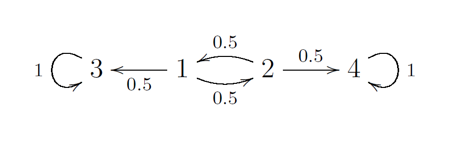
which gives us the matrix $$P=\begin{pmatrix}0 & 0.5 & 0 & 0 \\ 0.5 & 0 & 0 & 0 \\ 0.5 & 0 & 1 & 0 \\ 0 & 0.5 & 0 & 1\end{pmatrix}.$$ We view this matrix as consisting of four matrix blocks $$P=\begin{pmatrix}Q & 0 \\ R & I\end{pmatrix},$$ where in this case $$Q=\begin{pmatrix}0 & 0.5 \\ 0.5 & 0\end{pmatrix}, R = \begin{pmatrix} 0.5 & 0 \\ 0 & 0.5 \end{pmatrix},\mbox{ and } I=\begin{pmatrix}1 & 0 \\ 0 & 1\end{pmatrix}$$

Note that, for an arbitrary absorbing Markov chain, $Q$ is always a square matrix, $I$ is a square identity matrix which can be of a different size than $Q$, and that $R$ need not be square.

Using this blocking we can compute $$P^n=\begin{pmatrix}Q^n & 0\\ R(I+Q+\cdots+Q^{n-1}) & I\end{pmatrix}$$ which in the limit $n\rightarrow \infty$ is equal to $$lim_{n\rightarrow \infty}P^n=\begin{pmatrix}0 & 0 \\ RN & I\end{pmatrix}.$$ Of course, that $Q^n\rightarrow 0$ when $n\rightarrow \infty$ is not completely obvious and does require a proof. A consequence, however, is that any random walk will eventually lead to an absorbing state. The matrix $N=I+Q+Q^2+\cdots$ is called the fundamental matrix of the absorbing chain.

We will need to compute the fundamental matrix $N$. Notice that $$(I-Q)\cdot(I+Q+Q^2+\cdots) = I,$$ and so $(I-Q)$ is the inverse of $N$. So the preferred approach is to compute $$N=(I-Q)^{-1}.$$

From the matrices $N$ and $R$ we can for instance compute

$N[i][j]$ which is the expected number of times we will visit $i$ before absorption, when we start at $j$.
$R\cdot N[i][j]$ which is the probability that we will end up in state $i$ at absorption, when we start at $j$.
$c\cdot N[:,j]$, where $c=(1,1,\cdots,1)$, which is the expected number of steps before absorption, when we start at $j$.

The notation $N[:,j]$ is not mathematical, but is instead Python syntax for the $j$'th column in $N$. Links on Blackboard will lead you to information about computing other quantities.

We look a little bit more carefully at the first of these formulas, and skip the explanation of the other two. This explanation is really beyond what is required in the course, but included here because of requests in earlier years. Assume we are doing a random walk, starting at vertex $j$. Let $X_t$ be the random variable which is equal to $1$ if we end up at $i$ after $t$ steps and equal to $0$ otherwise. Since $X_t$ is Bernoulli, we have $E(X_t)=Q^t[i][j]$. Using that expectation commutes with sums we have $$E(X_0+\cdots +X_t) = Q^0[i][j] + \cdots + Q^t[i][j].$$ This number is the expected number of times we visit $j$ if we start at $i$ in $t$ steps. If we now let $t\rightarrow \infty$ we get that $N[i][j]$ is the expected number of times we will visit $i$ before absorption, when we start at $j$.

We end with an example computation in Python. We first create all the necessary matrices

import numpy as np

# the transition matrix
P = np.array([[0,0.5,0,0],[0.5,0,0,0],[0.5,0,1,0],[0,0.5,0,1]], dtype=float)

# other matrices
Q = np.copy(P[0:2, 0:2])
R = np.copy(P[2:, 0:2])
N = np.linalg.inv(np.identity(2)-Q)
c = np.array([1,1])

The information we are interested in are obtained by printing

print(N)
print(np.dot(c,N))
print(np.dot(R,N))

Let us assume we start our walk in state $1$. By looking at the printout, we now know that we will we taking two steps on average before absorption, where we will visit state $1$ on average $1.33$ times and state $2$ on average $0.67$ times. There is a $66$ percent chance that we will end up in state $3$ when we are absorbed.

Ergodic Markov Chains

A Markov chain is called ergodic if there is some power of the transition matrix which has only non-zero entries. An irreducible Markov Chain is a Markov Chain with with a path between any pair of states. The following is an example of an ergodic Markov Chain

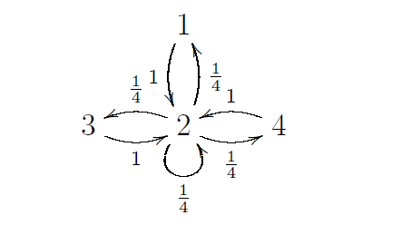
with transition matrix $$P=\begin{pmatrix}0 & \frac{1}{4} & 0 & 0\\ 1 & \frac{1}{4} & 1 & 1 \\ 0 & \frac{1}{4} & 0 & 0\\0 & \frac{1}{4} & 0 & 0\end{pmatrix}.$$ If you remove the loop at $2$ in this example, you will have an irreducible Markov chain, which is not ergodic.

For any irreducible Markov chain there is a vector $v$ with the properties

$P\cdot v = v$,
$\sum_i v[i]=1$, and
$v[i]\geq 0$ for all $i$.

Vectors with properties 2. and 3. are called probability vectors.

We can compute $v$ by solving the set of linear equations formed by the first two properties.

Let $W$ be the square matrix with columns equal to $v$. This matrix is equal to $$W=lim_{n\rightarrow \infty}\frac{1}{n+1}\sum^n_{i=0}P^i$$ which gives us another way to find $v$. When the Markov chain is ergodic, we also have $P^n\rightarrow W$ as $n\rightarrow \infty$, and $P^n\cdot x\rightarrow v$ as $n\rightarrow \infty$, for any choice of probability vector $x$.

The fundamental matrix of an ergodic chain is $$Z=(I-P+W)^{-1}.$$ Note that we use the name "fundamental matrix" for both absorbing chains an ergodic chains, but that these matrices are defined differently for these two types of chains.

The expected number of steps needed to move from state $i$ to state $j$ is the number $$M[i][j]=\frac{Z[i][i]-Z[i][j]}{v[i]}.$$ We see that $M[i][i]=0$ which tells us that zero steps are needed to move from state $i$ to state $i$. If we want to calculate the expected number of turns needed to move from state $i$ to state $i$, where we leave state $i$, then the number we want is $\frac{1}{v[i]}$. The entry $W[i][j]=v[i]$ computes the proportion of turns we will be at state $i$ when the length of the walk goes to infinity. Note that this number is independent of where the walk starts.

Random Walks on graphs

A random walks on a graph is a type of Markov Chain which is constructed from a simple graph by replacing each edge by a pair of arrows in opposite direction, and then assigning equal probability to every arrow leaving a node. In other words, the non-zero numbers in any column of the transition matrix are all equal. The example above is a random walk on a graph.

For a random walk on a graph we can read of the vector $v$ directly from the transition matrix. For example, for the Markov Chain above we have the following pieces of information:

There is $1$ node pointing to the node $1$,
There are $4$ nodes pointing to the node $2$.
There is $1$ node pointing to the node $3$.
There is $1$ node pointing to the node $4$.

The numbers $1,4,1,1$ and the sum $1+4+1+1=7$ gives us the probability vector $$v=\frac{1}{7}\begin{pmatrix}1&4&1&1\end{pmatrix}.$$ This method works in general for random walks on graphs.

An example

We analyse the Markov Chain

with transition matrix $$P=\begin{pmatrix}0 & \frac{1}{4} & 0 & 0\\ 1 & \frac{1}{4} & 1 & 1 \\ 0 & \frac{1}{4} & 0 & 0\\0 & \frac{1}{4} & 0 & 0\end{pmatrix}.$

We first create the adjancency matrix and compute the vector $v$ and the matrix $W$.

P = np.array([[0,1,0,0],[1,1,1,1],[0,1,0,0],[0,1,0,0]], dtype = float)
v = [sum(P[i]) for i in range(4)]
W = np.array([v for i in range(4)])
v = np.transpose((np.array(v) / sum(v)))
W = np.transpose(W)

We then compute the transition matrix, the fundamental matrix and the matrix $M$

P = np.transpose(np.array([P[i] / sum(P[i]) for i in range(4)]))
Z = np.linalg.inv(np.identity(4) - P + W)
M = np.zeros((4,4), dtype=float)
for i in range(4):
for j in range(4):
M[i][j] = (Z[i][i]-Z[i][j]) / v[i]

Finally, some information is printed to the screen

print(v)
print([1/v[i] for i in range(4)])
print(M)

From this we learn for instance that $57$ per cent of a long random walk will be spent in state $2$, and $14$ per cent will be spent at state $1$. We will need $7$ steps on average to return to state $3$ if we leave that state, and we also need $7$ steps on average to move from state $3$ to state $1$.